KotlinDL 0.4 Is Out With Pose Detection API, EfficientDet for Object Detection, and EfficientNet for Image Recognition
Version 0.4 of our deep learning library, KotlinDL, is out!
KotlinDL 0.4 is now available on Maven Central with a variety of new features – check out all of the changes that are coming to the new release! We’re currently introducing new models in ModelHub (including the EfficientNet and EfficientDet model families), the experimental high-level Kotlin API for Pose Detection, new layers and preprocessors contributed by the community members, and many other changes.
In this post, we’ll walk you through the changes to the Kotlin Deep Learning library in the 0.4 release:
- Pose Detection
- NoTop models in the ModelHub
- New models: EfficientDet and EfficientNet
- Multiple callbacks
- Breaking changes in the Image Preprocessing DSL
- 4 new layers and 2 new activation functions
- Learn more and share your feedback
Pose Detection
Pose detection is using an ML model to detect the pose of a person from an image or a video by detecting the spatial locations of key body joints (keypoints).
We’re excited to launch the MoveNet family of pose detection modes with our new pose detection API in KotlinDL. MoveNet is a fast and accurate model that detects 17 keypoints on the body. The model is offered on ONNXModelHub with two variants, MoveNetSinglePoseLighting and MoveNetSinglePoseThunder. MoveNetSinglePoseLighting is intended for latency-critical applications, while MoveNetSinglePoseThunder is intended for applications that require high accuracy.
If you need to detect a few poses on a given image or video frame, try MoveNetMultiPoseLighting. This model is able to detect multiple people in the image frame at the same time, while still achieving real-time speed.
There are two ways to detect poses within the KotlinDL: parsing the model output manually or using our LightAPI for Pose Detection (the recommended way).
Just load the model:
val modelHub = ONNXModelHub(cacheDirectory = File("cache/pretrainedModels"))
val model = ONNXModels.PoseDetection.MoveNetSinglePoseLighting.pretrainedModel(modelHub)
Run the predictions and print out the pose landmarks and edges connecting the detected pose landmarks:
model.use { poseDetectionModel ->
       val imageFile = …
       val detectedPose = poseDetectionModel.detectPose(imageFile = imageFile)

       detectedPose.poseLandmarks.forEach {
           println("Found ${it.poseLandmarkLabel} with probability ${it.probability}")
       }

       detectedPose.edges.forEach {
           println("The ${it.poseEdgeLabel} starts at ${it.start.poseLandmarkLabel} and ends with ${it.end.poseLandmarkLabel}")
       }
}
Some visualization examples, where we drew landmarks and edges on the given images, are below.
The complete example can be found here.
If you want to run the MoveNet model to detect multiple poses on the given image, you need to make some minor changes to your code.
First, load the model:
val modelHub = ONNXModelHub(cacheDirectory = File("cache/pretrainedModels"))
val model = ONNXModels.PoseDetection.MoveNetSinglePoseLighting.pretrainedModel(modelHub)
Secondly, run the model and get the MultiPoseDetectionResult object, which contains the list of pairs <DetectedObject, DetectedPose>. As a result, we have access not only to the landmarks’ coordinates and labels, but also to the coordinates of the bounding box for the whole person.
model.use { poseDetectionModel ->
       val imageFile = …
       val detectedPoses = poseDetectionModel.detectPoses(imageFile = imageFile, confidence = 0.0f)

       detectedPoses.multiplePoses.forEach { detectedPose ->
           println("Found ${detectedPose.first.classLabel} with probability ${detectedPose.first.probability}")
           detectedPose.second.poseLandmarks.forEach {
               println("Found ${it.poseLandmarkLabel} with probability ${it.probability}")
           }

           detectedPose.second.edges.forEach {
               println("The ${it.poseEdgeLabel} starts at ${it.start.poseLandmarkLabel} and ends with ${it.end.poseLandmarkLabel}")
           }
       }
}
Some visualization examples, where we drew the bounding boxes, landmarks, and edges on the images are below.
The complete example can be found here.
NoTop models in the ModelHub
Running predictions on ready-made models is good, but what about fine-tuning them for your tasks?
The classic approach to Transfer Learning is to freeze all layers except the last few and then train the top few layers (the fully connected layers at the top of the network) on a new piece of data, often changing the number of model outputs.
Before the 0.4 release, KotlinDL users needed to remove the last layers manually, but with the 0.4 release, TensorFlowModelHub provides an option to download “noTop” models – equivalent to earlier available models, but without weights and configurations for the last few layers.
The following “noTop” models are now available:
- VGG’16
- VGG’19
- ResNet50
- ResNet101
- ResNet152
- ResNet50V2
- ResNet101V2
- ResNet152V2
- MobileNet
- MobileNetV2
- NasNetMobile
- NasNetLarge
- DenseNet121
- DenseNet169
- DenseNet201
- Xception
- Inception
In the example below, we load the ResNet50 model from our TensorFlowModelHub and fine-tune it to classify cats and dogs (using the embedded Dogs-vs-Cats dataset):
val modelHub = TFModelHub(cacheDirectory = File("cache/pretrainedModels"))

val modelType = TFModels.CV.ResNet50(noTop = true, inputShape = intArrayOf(IMAGE_SIZE, IMAGE_SIZE, NUM_CHANNELS))

val noTopModel = modelHub.loadModel(modelType)
The topModel is the simplest neural network and can be trained quickly, as it has few parameters.
val topModel = Sequential.of(
   GlobalAvgPool2D(
       name = "top_avg_pool",
   ),
   Dense(
       name = "top_dense",
       kernelInitializer = GlorotUniform(),
       biasInitializer = GlorotUniform(),
       outputSize = 200,
       activation = Activations.Relu
   ),
   Dense(
       name = "pred",
       kernelInitializer = GlorotUniform(),
       biasInitializer = GlorotUniform(),
       outputSize = NUM_CLASSES,
       activation = Activations.Linear
   ),
   noInput = true
)
The new helper function could join two models together: noTop and topModel: val model = Functional.of(pretrainedModel = noTopModel, topModel = topModel)
After that, load weights for the frozen layers from the noTop model, and the weights for the unfrozen layers from the topModel will be initialized during the fit method call.
model.use {
   it.compile(
       optimizer = Adam(),
       loss = Losses.SOFT_MAX_CROSS_ENTROPY_WITH_LOGITS,
       metric = Metrics.ACCURACY
   )

   it.loadWeightsForFrozenLayers(hdfFile)

   it.fit(
       dataset = train,
       batchSize = TRAINING_BATCH_SIZE,
       epochs = EPOCHS
   )

   val accuracy = it.evaluate(dataset = test, batchSize = TEST_BATCH_SIZE).metrics[Metrics.ACCURACY]

   println("Accuracy: $accuracy")
}
The complete example can be found here.
New models: EfficientDet and EfficientNet
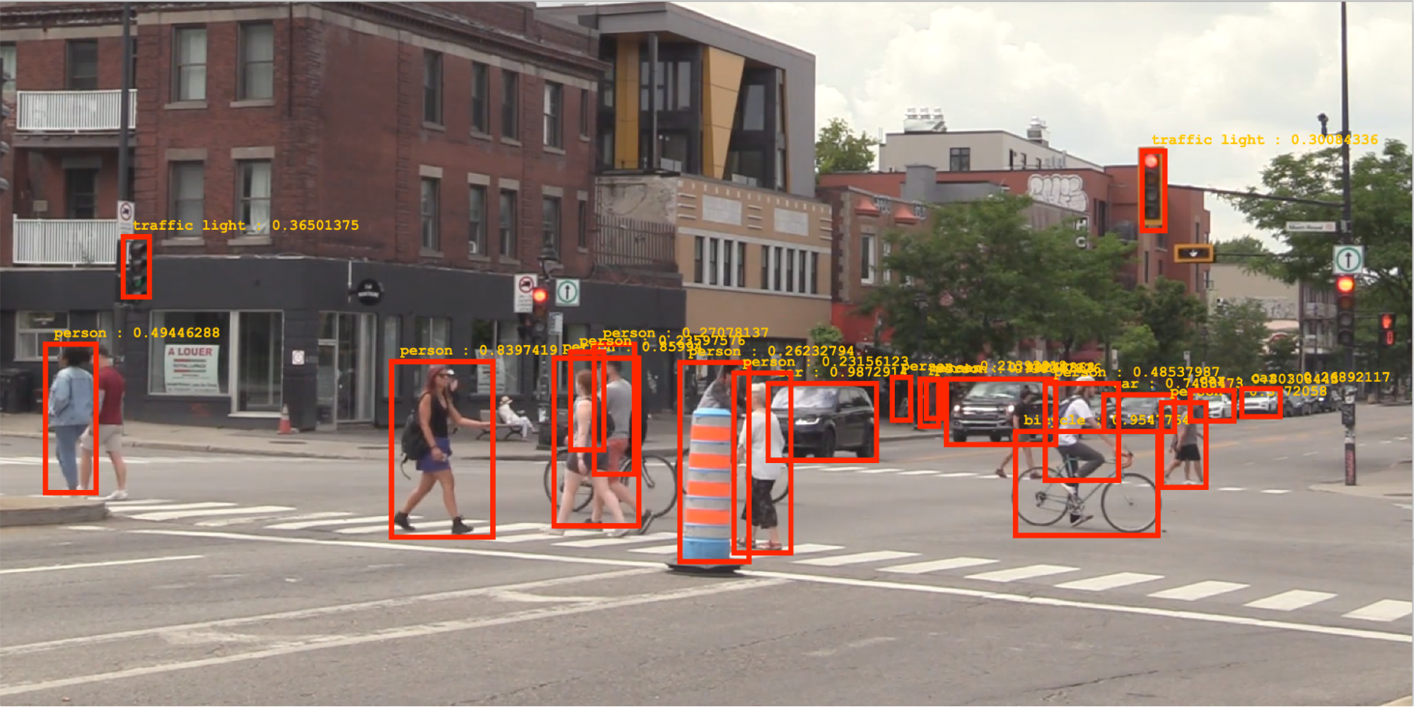
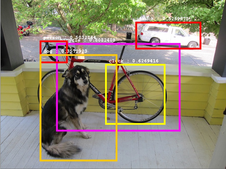
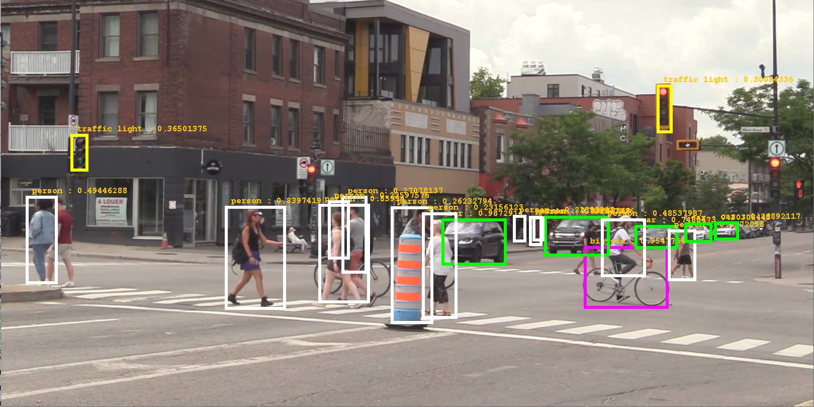
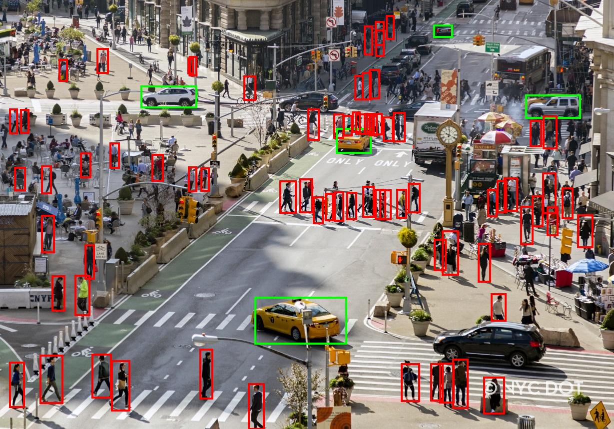
Until v0.4, our ModelHub contained only one model (SSD) suitable for solving the Object Detection problem. Starting with this release, we’re gradually expanding the library’s capabilities for solving the Object Detection problem. We’d like to introduce to you a new family of object detectors, called EfficientDet, which consistently achieve much better efficiency than prior object detectors across a wide spectrum of resource constraints.
All models from this family have the same internal architecture which scales for different inputs (image resolution). The final user has a choice of models: from the smallest EfficientDet-D0, model with 3.9 million parameters and 10.2 ms latency on the V100 up to the EfficientDet-D7, with 52 million parameters and 122 ms latency on the V100.
Internally, EfficientDet models use another famous model, EfficientNet, as a backbone. It extracts features from input images and passes them to the next component of the Object Detection model).
An example of EfficientDet-D2 usage can be found here.
The EfficientNet model family is also available in the ONNXModelHub. There are 8 different types of models and each model is presented in two variants: full and “noTop” for fine-tuning.
These models achieve better accuracy on the ImageNet dataset with 10x fewer parameters than ResNet or NasNet. If you need fast and accurate image recognition, EfficientNet is a good choice.
An example of EfficientNet0 usage can be found here.
Multiple callbacks
Earlier, Callback support for KotlinDL was pretty simple and not fully compatible with Keras. As a result, users faced difficulties in implementing their neural networks, building the custom validation process, and monitoring the neural network’s training.
The callback object was passed during compilation and was unique for each stage in the model’s lifecycle. However, model compilation can be located in very different places in the code than fit/predict/evaluate, meaning that users may need to create different callbacks for different purposes.
Let’s assume that we need to define EarlyStopping and TerminateOnNaN for training to handle exceptional cases, and also add two custom callbacks for the prediction and evaluation phases:
val earlyStopping = EarlyStopping(
   monitor = EpochTrainingEvent::valLossValue,
   minDelta = 0.0,
   patience = 2,
   verbose = true,
   mode = EarlyStoppingMode.AUTO,
   baseline = 0.1,
   restoreBestWeights = false
)
val terminateOnNaN = TerminateOnNaN()


class EvaluateCallback : Callback() {
   override fun onTestBatchEnd(batch: Int, batchSize: Int, event: BatchEvent?, logs: History) {
       println("Test batch $batch ends with loss ${event!!.lossValue}..")
   }

   override fun onTestEnd(logs: History) {
       println("Train ends with last loss ${logs.lastBatchEvent().lossValue}")
   }
}

class PredictCallback : Callback() {
   override fun onPredictBatchBegin(batch: Int, batchSize: Int) {
       println("Prediction batch $batch begins.")
   }

   override fun onPredictBatchEnd(batch: Int, batchSize: Int) {
       println("Prediction batch $batch ends.")
   }
}
Let’s pass these callbacks to the model methods:
model.use {
   it.compile(
       optimizer = Adam(clipGradient = ClipGradientByValue(0.1f)),
       loss = Losses.SOFT_MAX_CROSS_ENTROPY_WITH_LOGITS,
       metric = Metrics.ACCURACY
   )

   it.logSummary()

   it.fit(
       dataset = train,
       epochs = EPOCHS,
       batchSize = TRAINING_BATCH_SIZE,
       callbacks = listOf(earlyStopping, terminateOnNaN)
   )

   val accuracy = it.evaluate(
       dataset = test,
       batchSize = TEST_BATCH_SIZE,
       callback = EvaluateCallback()
   ).metrics[Metrics.ACCURACY]


   val predictions = it.predict(
       dataset = test,
       batchSize = TEST_BATCH_SIZE,
       callback = PredictCallback()
   )
}
Found below in the logs:
The complete example can be found here.
4 new layers and 2 new activation functions
Many contributors to this release have added layers to Kotlin for performing non-trivial logic. With these added layers, you can start working with autoencoders and load the GAN models:
- Dot layer (by Ansh Tyagi)
- Conv1DTranspose, Conv2DTranspose, and Conv3DTranspose layers (by Julia Beliaeva)
There are also two new activation functions:
- Sparsemax activation function (by Cagri Yildirim)
- Soft shrink activation function (by Michal Harakal)
These activation functions are not available in the TensorFlow core package, but we decided to add them after seeing how they’ve been widely used in recent papers.
We’d be delighted to look at your pull requests if you’d like to contribute a layer, activation function, callback, or initializer from a recent paper!
Breaking changes in the Image Preprocessing DSL
There are a few major changes in the Image Preprocessing DSL:
- CustomPreprocessor was removed.
- The loading section was moved from image preprocessing to the Dataset API
- A few new Preprocessors were added:
- Padding
- CenterCrop
- Convert
- Grayscale
- Normalizing
Here is an example of some of the new operations:
val preprocessing = preprocess {
 transformImage {
   centerCrop {
     size = 214
   }
   pad {
     top = 10
     bottom = 10
     left = 10
     right = 10
     mode = PaddingMode.Fill(Color.BLACK)
   }
   convert {
     colorMode = ColorMode.BGR
   }
 }
 transformTensor {
   normalize {
     mean = floatArrayOf(103.939f, 116.779f, 123.68f)
     std = floatArrayOf(57.375f, 57.12f, 58.395f)
   }
 }
}
Because of the removal of the loading section, the same preprocessing instance could now be used in several datasets:
val trainDataset = OnHeapDataset.create(File(datasetPath, "train"), labelGenerator, preprocessing)
val valDataset = OnHeapDataset.create(File(datasetPath, "val"), labelGenerator, preprocessing)
Standing on the shoulders of giants
We’d like to express our deep gratitude to Alexey Zinoviev for his great work developing the framework from minimum viable product to the current state, efforts towards creating a community, skillful release management, and competent marketing support.
His passion for democratizing AI and his continuous work to improve the ability of Kotlin and Java developers to use ML/DL models deserves great respect and inspires us to continue our work.
We’d also like to express our gratitude to Veniamin Viflyantsev, who’s invested a lot of time and effort into changing the architecture of the api module. Many of his changes are now part of this release.
Our team has expanded! Julia Beliaeva (author of the new version of Image Preprocessing DSL) and Nikita Ermolenko have joined us on a permanent basisWe wish them good luck and look forward to new releases!
Learn more and share your feedback
We hope you enjoyed this brief overview of the new features in KotlinDL 0.4! For more information, including the up-to-date Readme file, visit the project’s home on GitHub. Be sure to check out the KotlinDL guide, which contains detailed information about the library’s basic and advanced features and covers many of the topics mentioned in this blog post in more detail.
If you’ve previously used KotlinDL, use the changelog to find out what has changed and how to upgrade your projects to the stable release.
We’d be very thankful if you’d report any bugs you find to our issue tracker. We’ll try to fix all of the critical issues in the 0.4.1 release.
You’re also welcome to join the #kotlindl channel in Kotlin Slack (get an invite here). In this channel, you can ask questions, participate in discussions, and get notifications about the new preview releases and models in ModelHub.