Multik 0.2: Multiplatform, With Support for Android and Apple Silicon
Introducing Multik 0.2.0! Now a multiplatform library, it allows you to use multidimensional arrays in your favorite multiplatform projects. Let’s take a closer look at what’s new in v0.2.0.
Multiplatform
We are very grateful to Luca Spinazzola for his huge contribution to the multiplatform capabilities included in this release of the library.
Before we move on to reviewing Multik’s new multiplatform structure, we need to say a few words about the new naming conventions. Ever since we multiplied the number of artifacts and added platform suffixes, such as jvm, macosx64, js, and others, there have been collisions with older names. To solve this problem, we’ve renamed some of the modules.
Let’s reacquaint ourselves with the modules and get a sense of which platforms each module now supports.

multik-core
As the name suggests, this is the main module providing multidimensional arrays and the ability to perform transformations, iteration, and arithmetic operations with them. This module also provides an API for calculations that require complex algorithms and resources. Now there are three types of such APIs: mathematics, linear algebra, and statistics. Other modules are responsible for the implementation of this API. Remember – Multik lets you replace these implementations at runtime.
We have added support for all major platforms for this module. Note that JavaScript uses a new IR and Kotlin/Native uses a new memory model, so these artifacts will only be compatible with projects that support them.
multik-core |
multik-kotlin |
multik-openblas |
multik-default |
|
| jvm | ✓ | ✓ | ✓ linuxX64 ✓ mingwX64 ✓ macosX64 ✓ macosArm64 ✓ androidArm64 |
✓ linuxX64 ✓ mingwX64 ✓ macosX64 ✓ macosArm64 ✓ androidArm64 |
| linuxX64 | ✓ | ✓ | ✓ | ✓ |
| mingwX64 | ✓ | ✓ | ✓ | ✓ |
| macosX64 | ✓ | ✓ | ✓ | ✓ |
| macosArm64 | ✓ | ✓ | ✓ | ✓ |
| iosArm64 | ✓ | ✓ | ✕ | ✓ |
| iosX64 | ✓ | ✓ | ✕ | ✓ |
| iosSimulatorArm64 | ✓ | ✓ | ✕ | ✓ |
| js | ✓ | ✓ | ✕ | ✓ |
multik-kotlin
The first module that implements the above API is multik-kotlin. In this module, all algorithms and logic are written in pure Kotlin. Even though it may be slower than native libraries, it provides more stability and allows for easier code debugging.
Because everything is written in Kotlin, it was also possible to support most of the important platforms, including JVM, Desktop, iOS, and JavaScript.
multik-openblas
The next module is multik-openblas. Here, the OpenBLAS library is responsible for all linear algebra as well as the C wrapper over the Fortran libraries LAPACK and BLAS. C++ code is responsible for mathematics and statistics.
This module, unlike the previous one, is quite demanding on the environment and the platform it’s launched on. In the table, you can see that the code under the JVM will only work on the specified systems and architectures. On these platforms, we ensure that it works out of the box and the users are rewarded with excellent performance.
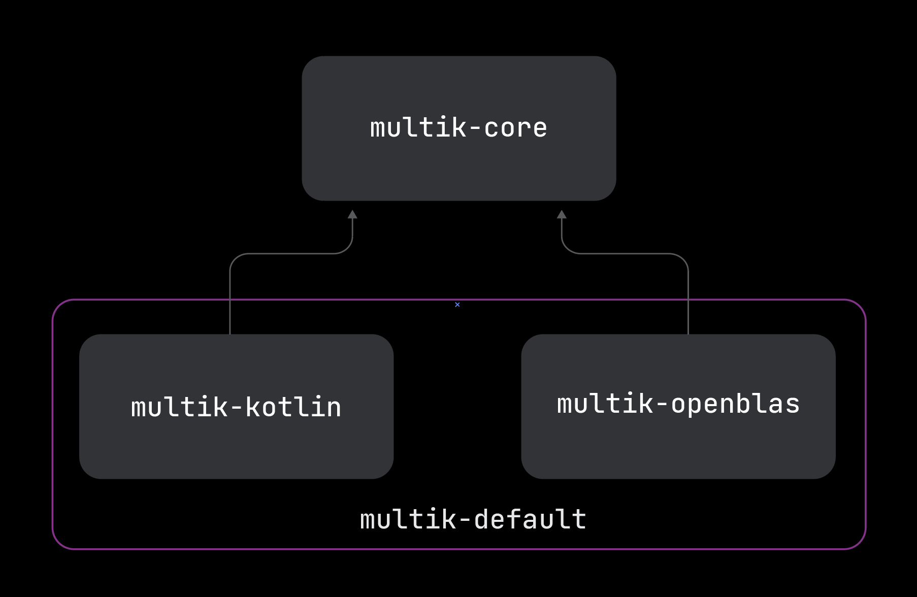
multik-default
multik-default, the last of the 4 models available at the moment, has kept its old name. It includes the two previous modules, multik-kotlin and multik-openblas. The idea is to combine the pros of both modules while doing away with the cons.
It supports all of the same platforms as the previous modules.
Support for Android and Apple Silicon processors
multik-openblas is supported by Android and macOS on new Apple processors. Now you can enjoy the speed of applications on Android with ARMv8 processors and native support for M1 and M2 processors from Apple.
Random, norm matrix, easy creation of complex numbers, and more
In this release, we have also improved the usability of the library. For example, we wrapped random from Kotlin to create arrays with random numbers:
val ndarray = mk.rand<Float>(3, 5, 2)
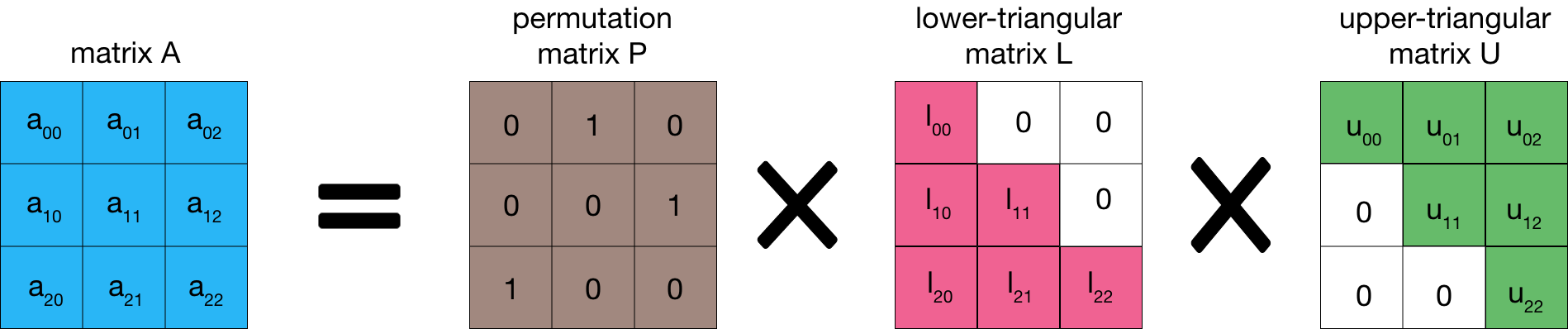
We have changed the matrix norm calculation function and added it to the native one:
val ndarray = mk.ndarray(mk[mk[1.0, 2.0], mk[3.0, 4.0]])
mk.linalg.norm(ndarray)
mk.linalg.norm(ndarray, Norm.Inf)
And now you can create complex numbers easily and naturally. Credit for this contribution goes to Marcus Dunn.
val complexNumber: ComplexDouble = 1.0 + 1.0.i
For more details about this new release, please check out the changelog.
How to try it
To try Multik 0.2.0 in your project, do the following:
- Make sure that you have
mavenCentral()in your list of repositories:
repository {
    mavenCentral()
}
- Add the Multik module you need as a dependency:
dependencies {
    implementation("org.jetbrains.kotlinx:multik-core:0.2.0")
}
For a multiplatform project, put the Multik dependency in the common set:
commonMain{
   dependencies {
       implementation("org.jetbrains.kotlinx:multik-core:0.2.0")
   }
}
Or put the dependency in a specific source set.
Multik is also available in Kotlin Jupyter notebooks.
%use multik
Try it in Datalore.
Conclusion
We are on our way to a stable release and could really use your feedback.
Try out Mutlik 0.2.0 and share your experience with us! Report any issues you encounter to the project’s issue tracker.